Learning Haskell
15 Jun, 2016
Haskell is a functional programming language, very different to the programming languages I'm used to (C++, Python, JavaScript...). I've been hearing about Haskell for a while; people emphasize its elegance, its mathematical inspiration and foundation, and the fact that being based on such a different paradigm with respect to imperative programming it helps thinking about programming from a very different perspective. Python, Java, C++... are all languages that are incorporating concepts from functional programming to their latest versions. Therefore I was willing to learn some Haskell.
 Haskell logo
Material
I began to look for books, tutorials, presentations, etc. For me, the best book for beginners is Learn You a Haskell for Great Good!. This presentation (in Spanish) by UJI professor Andrés Marzal is also very interesting and entertaining (in two hours and a half he starts presenting Haskell and ends up explaining some pretty advanced features), it also includes some great pdf notes. I also checked the book Real World Haskell, which I don't think is the best book to start with, but it surely has very interesting information if you want to develop larger projects.
Practice with... the Judge!
Once I was convinced of the benefits of Haskell, I wanted to start writing some code, but did not have any project in mind. That's when I thought of learning Haskell the same way I had learned to program in C++ many years ago: with the Judge.
 The Judge with the classic traffic light:
green or red depending on whether your program is correct or not.
The Judge with the classic traffic light:
green or red depending on whether your program is correct or not.
The Judge is a platform to learn how to program, developed by professors Jordi Petit and Salvador Roura at UPC. This platform contains problems to be solved by programs that are sent to the same Judge, which automatically checks whether their execution is correct. The Judge is used in many UPC programming and algorithms courses and its use is open to the public, even more... it contains 33 problems of a Haskell programming course!
Thus, in recent weeks I have done these 33 problems :-). It has been a very fun experience and a great excercise to get familiar with the language and the development environment.
Haskell examples
Next I'll show some Haskell features to give an idea of its potential. These concepts are explained in more depth in Learn You a Haskell for Great Good!, here I will present them together with some code examples.
Working in Ubuntu, you can install haskell-platform (sudo apt-get install
haskell-platform) and use the ghci interpreter. You can save the programs in
files (e.g. prog.hs), defining in them the funtions you want. Then, these
functions can be loaded (and reloaded) with ghci>: l to prog, which makes
them available to be used and tested.
Let's see which are these interesting Haskell functionalities...
Recursion
Haskell, as a functional programming language, doesn't have loops: no while,
no for. One way to implement what could be done using loops is through
recursion. An example with the factorial function:
$$factorial(n) = n! = n\cdot (n-1)\cdots2\cdot 1$$
Recursively, we could define it as:
$$\begin{cases} factorial(0) = 1 \\ factorial(n) = n\cdot factorial(n-1) \end{cases}$$
And in Haskell, it could be implemented as follows:
factorial :: Integer -> Integer
factorial 0 = 1
factorial n = n * factorial (n-1)
The first line is the signature of function, which specifies the type of the
parameter and result. In our case, we use Integer, which are integer numbers
of arbitrary length.
Lists
Many programs need to work with lists of values, and Haskell offers us many ways to do it comfortably. For example, let's see some ways to get even numbers between 0 and 20:
Prelude> [2,4..20]
[2,4,6,8,10,12,14,16,18,20]

Prelude> filter even [1..20]
[2,4,6,8,10,12,14,16,18,20]

Prelude> [x | x <- [1..20], even x]
[2,4,6,8,10,12,14,16,18,20]
Note the last expression, which is a list comprehension, very similar to the mathematical notation $\left\{x \; \vert \; \forall\, x \in {1,\ldots,20},\; iseven(x)\right\}$.
Using recursion and list comprehensions we can implement the quicksort sorting algorithm. Given a list, quicksort orders the items as follows:
- Choose the first element as a pivot.
- Build two lists: the first with elements smaller than the pivot, and the second with elements bigger than the pivot.
- Sort these two lists using the same quicksort algorithm.
- The result is a list containing the sorted smaller values, followed by the pivot, followed by the sorted list of bigger values.
The Haskell implementation of this algorithm can be very neat:
qsort :: [Int] -> [Int]
qsort [] = []
qsort (x:xs) =
    qsort [y | y <- xs, y <= x] ++ [x] ++ qsort [y | y <- xs, y > x]
Lazy evaluation
Haskell is based entirely on the lazy evaluation, ie, making the calculations as late as possible, and that's when they are needed by someone else. This enables the language to use endless lists, because values of the list are only calculated when another task needs them. For example:
Prelude> take 5 [1 ..]
[1,2,3,4,5]

Prelude> take 10 [1 ..]
[1,2,3,4,5,6,7,8,9,10]
Using this feature, we can implement the sieve of Eratosthenes algorithm, which generates the list of prime numbers.
The sieve of Eratosthenes begins with number 2 (which is prime) and marks all its multiples. It repeatedly takes the smallest number not marked, which is prime because it is no a multiple of any other smaller number, and again marks all of its multiples.
This process returns all primes smaller than a given number: obviously we can not mark all even numbers, because they never end. Moreover, what we can do is to discard all even numbers lower than 1000, for example. Haskell, however, by using lazy evaluation, is able to work with never ending lists and therefore allows a very simple implementation:
primes :: [Int]
primes = sieve [2..]
    where
        sieve (p:xs) = p : sieve [x | x <- xs, x `mod` p > 0]
We save it in the file primes.hs and we can run:
$ ghci
GHCi, version 7.6.3: http://www.haskell.org/ghc/  :? for help

Prelude> :l primes
[1 of 1] Compiling Main             ( primes.hs, interpreted )
Ok, modules loaded: Main.

*Main> take 5 primes
[2,3,5,7,11]

*Main> takeWhile (<50) primes
[2,3,5,7,11,13,17,19,23,29,31,37,41,43,47]
Higher order functions
Higher order functions are functions that take other functions as parameters.
An example is the map function, which takes a function as the first parameter
and a list as the second parameter, and it applies the function to each item in
the list. For example:
Prelude> map (* 2) [1..10]
[2,4,6,8,10,12,14,16,18,20]

Prelude> map (^ 2) [1..10]
[1,4,9,16,25,36,49,64,81,100]
Given a list of integers, and a list of exponents, we can raise each number to the given power:
Prelude> zipWith (^) [1..5] [1..5]
[1,4,27,256,3125]
Here You can find more examples of higher order functions and their use.
Pattern matching
Another interesting feature of Haskell is pattern matching. We can check the
pattern (x:y:xs) over a list, so x and y represent the first and second
value of the list and xs the remaining elements.
Let us see how we can use pattern matching to implement binary tree traversal in different orders. Let's remember first preorder, inorder and postorder traversals:
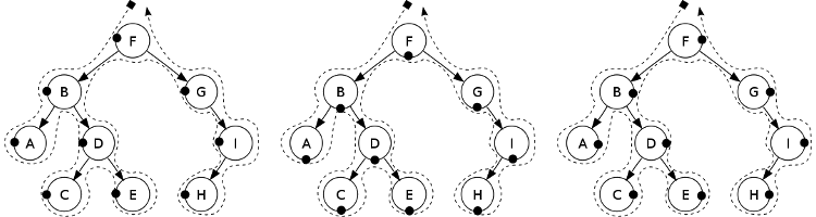 *
Ways to traverse a binary tree: preorder (left: F, B, A, D, C, E, G, I, H)
inorder (center: A, B, C, D, E, F, G, H, I) and postorder (right: A, C, E, D,
B, H, I, G, F). The black dots indicate at what time of the route each node is
chosen*
*
Ways to traverse a binary tree: preorder (left: F, B, A, D, C, E, G, I, H)
inorder (center: A, B, C, D, E, F, G, H, I) and postorder (right: A, C, E, D,
B, H, I, G, F). The black dots indicate at what time of the route each node is
chosen*
And that we can implement it like this:
data Tree a = Node a (Tree a) (Tree a) | Empty deriving (Show)

preOrder :: Tree a -> [a]
preOrder Empty = []
preOrder (Node n t1 t2) = [n] ++ preOrder t1 ++ preOrder t2

postOrder :: Tree a -> [a]
postOrder Empty = []
postOrder (Node n t1 t2) = postOrder t1 ++ postOrder t2 ++ [n]

inOrder :: Tree a -> [a]
inOrder Empty = []
inOrder (Node n t1 t2) = inOrder t1 ++ [n] ++ inOrder t2
The expressions (Node n t1 t2) is where pattern matching takes place.
Input / output
Consider also a small example of input/output: a program that reads the name
a person says Hello maca if the name ends in a and Hello maco
otherwise (maco and maca mean pretty in Catalan :P):
main :: IO()
main = do
    name <- getLine
    putStrLn $
        "Hola mac" ++
        (if elem (last name) "aA" then "a" else "o") ++ "!"
Product of polynomials with Fast Fourier Transform
Finally, let's see the implementation of polynomial multiplication using the Fast Fourier Transform. The product of polynomials of degree $n$ has a cost of $\mathcal{O}(n^2)$ if we use the trivial algorithm: we multiply each coefficient of the first polynomial by each coefficient of the second polynomial, and then add them as needed, which leads to a quadratic performance. There is a much faster algorithm with a performance of $\mathcal{O}(n\log n)$, which uses the Fast Fourier Transform.
A very good explanation of how this algorithm works and how to implement it can be found here.
Next I show a working implementation, where the FFT is implemented in only 12 lines of code and 10 more lines are used to implement polynomial multiplication.
import Data.Complex

fft :: [Complex Double] -> Complex Double -> [Complex Double]
fft [a] _ = [a]
fft a w = zipWith (+) f_even (zipWith (*) ws1 f_odd) ++
          zipWith (+) f_even (zipWith (*) ws2 f_odd)
    where
        -- Take even and odd coefficients of a(x)
        a_even = map fst $ filter (even . snd) (zip a [0..])
        a_odd  = map fst $ filter (odd  . snd) (zip a [0..])
        -- Compute FFT of a_even(x) and a_odd(x) recursively
        f_even = fft a_even (w^2)
        f_odd  = fft a_odd  (w^2)
        -- Compute 1st and 2nd half of unity roots (ws2 = - ws1)
        ws1 = take (length a `div` 2) (iterate (*w) 1)
        ws2 = map negate ws1

-- Multiplication of polynomials: c(x) = a(x) · b(x)
--     * a(x) and b(x) have degree n (power of 2), c(x) has degree 2n
--   Algorithm:
--     1. Compute f_a = fft(a), f_b = fft(b)  .. O(n·logn)
--     2. Compute product: f_c = f_a · f_c    .. O(n)
--     3. Interpolate c: c = fft^{-1}(f_c)    .. O(n·logn)
mult :: [Double] -> [Double] -> [Double]
mult [] _ = []
mult a b = map realPart c
    where
        n = length a
        w = exp (pi * (0 :+ 1) / fromIntegral n)
        f_a = fft (map (:+ 0) $ a ++ replicate n 0.0) w
        f_b = fft (map (:+ 0) $ b ++ replicate n 0.0) w
        f_c = zipWith (*) f_a f_b
        c = map (/ (fromIntegral $ 2*n)) $ fft f_c (1/w)
To test this program, save it in the file fft.hs, open a Haskell interpreter
ghci and load the program: :l fft.hs. We can multiply polynomials with
mult [2,1] [3,-2]. Because we are working with floating point numbers, we can
see small inaccuracies (eg. instead of 2.0, the system can save
1.9999999999999996). That's why we define round2, a function which rounds
numbers to two decimal places. Here are some examples:
$ ghci
GHCi, version 7.6.3: http://www.haskell.org/ghc/  :? for help

Prelude> :l fft.hs
[1 of 1] Compiling Main             ( fft.hs, interpreted )
Ok, modules loaded: Main.

*Main> let round2 f = (fromInteger $ round $ f * 100) / 100

*Main> map round2 $ mult [2,1] [3,-2]
[6.0,-1.0,-2.0,0.0]

*Main> map round2 $ mult [2,1,0,0] [3,-2,0,0]
[6.0,-1.0,-2.0,0.0,0.0,0.0,0.0,0.0]

*Main> map round2 $ mult [3.5,-2,6,1] [3.5,-2,6,1]
[12.25,-14.0,46.0,-17.0,32.0,12.0,1.0,0.0]

*Main> map round2 $ mult [1,2,3,4,5,6,7,8] [0,0,0,0,1,0,0,0]
[0.0,0.0,0.0,0.0,1.0,2.0,3.0,4.0,5.0,6.0,7.0,8.0,0.0,0.0,0.0,0.0]